Tooling
Explains the tools that are available to users.
- Tool Overview
- Select Features
- Measure Tool
- Burial Assessment
- Profile Tools
- Calculate Tools
- Markers
- 3D View
- Export Map to PDF
Tool Overview
| Icon | Tool |
 |
Select Features Select features within a specific region on the map. |
 |
Measure Measure the distance of a line or the surface of an area between two points. |
 |
Marker |
 |
Profiles |
 |
Burial (Difference) Assessment Calculates the (difference in) burial depth of a cable/pipeline relative to a single or combination of bathymetry layers. The result creates a new layer that shows the status as a color on top of the line. |
 |
|
 |
Display Options Adjust how raster layers are visualized on the map. |
 |
3D View Load a 3D visualization of a raster file and view/rotate/zoom it in a new browser tab. |
 |
Export Map Create a downloadable PDF chart. |
Select Features
Select features on a map to examine an object or area of interest in detail. Clicking the tool opens a context menu for selecting the shape of the region.
Select options
Choose whether you wish to view visible layers or all layers (including hidden layers):
| Icon | Select tool |
 |
Select with a rectangle shape. |
 |
Select with a circle shape. |
 |
Select with a custom polygon. |
 |
Show all layers (including hidden layers) or only visible vector layers. |
 |
Clear selection |
- Click on the starting point of the region.
- Click on the end point of the region (a polygon, which has multiple points, should finish on the starting point).
- The selection will automatically be highlighted on the map and in the layer manager.
- The attribute table in the context menu of a highlighted layer will show the selected features.
- The original tool button is changed in a clear selection button. Clicking it will cancel the selection.
Note
- If the region is within an area, it will be selected, although the selection is not expanded. Features in the area, but outside the selection region, are not selected.
- The attribute table will show only the selected features by default. Use the ‘’show all'' button to show features that have not been selected.
Measure Tool
| Icon | Measure Tool |
 |
Measure Area |
 |
Measure Distance |
 |
Clear measurements |
Measure Area
- The first click on the map sets the starting point.
- Each successive single click adds a point to the area polygon.
- Double clicking on a point adds the last point and measures the complete area.
- A new single click on the map starts the process of creating a new area to measure.
- The original tool button automatically changes into a ‘clear measurements' button (see below), which will clear all areas if clicked:
Measure Distance
- The first click on the map sets the starting point.
- Each successive single click adds a point to the line.
- Double-clicking on a point adds the last point. The length of the line is then measured.
- A new single click on the map starts a line measurement.
- The original tool button changes into a ‘clear measurements' button and will clear all lines:
Burial Assessment
Burial assessment 

The Burial Assessment Tool checks the distance between a cable or pipeline and a single bathymetry layer. It adds the result as a (temporary) layer in the calculations group in the layer manager.
The underlying data can be exported via the layer manager in different file formats (CSV, GeoJson, ShapeFile). It can also show the data in an attribute table, where each section of the line is shown. The layer shows the status as a color (red/yellow/green) on top of the line, as shown in the picture below.

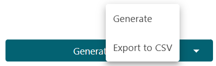
The results can be directly exported to a CSV instead of as a layer in the layer manager.
Options
| Option | Description |
| Cable/pipeline | Selects the cable/pipeline. |
| Bathymetry layer | Selects the layer with the seabed floor. |
| Criteria | Selects the criteria for OK/At Risk/Critical. An optional ‘small risk' level is also available. |
| KP | Optionally selects a section of the line instead of the full length of the line. This can be done with the slider or manually entering the start and end point. |
| Interval | Set the interval for points. The default is KP (kilometer points) as defined on the cable/pipeline. It is also possible to set a fixed distance between the points. |
CSV output format
The CSV is in XYZ format, each point on a cable has its own row.
Example
| CableName | X | Y | Z | KP | DoB | Status | Criteria |
| A1 | 497610.6 | 5730607 | -31.93 | 0 | AtRisk | [0.6m - 1m] | |
| A1 | 497609.4 | 5730597 | -31.96 | 0.01 | AtRisk | [0.6m - 1m] | |
| A1 | 497608.1 | 5730587 | -30.3 | 0.02 | Critical | <= 0.6m |
Burial Assessment Difference 


When cables and pipelines are buried under the seabed, tidal movements and other forces of nature change the depth at which they are buried. Understanding changes over time allows owners of subsea assets to plan the potential reburying of assets if necessary.
To use the Burial Assessment Difference Tool, select the surveys that you wish to compare. Calculate the difference between layer B against layer A above a cable or pipeline. A negative value (red) means less cover, a positive (green) means more cover. White, as shown between the two monopiles in the picture above, means no (noteworthy) difference.
Clicking the ‘’Generate" button will add the results to a (temporary) layer in the calculations group in the layer manager. The underlying data can be exported via the layer manager in different file formats (GeoJson, ShapeFile). It can also show the data in an attribute table, where each section of the line is shown. The layer shows the status as a color (red/white/green) on top of the line.
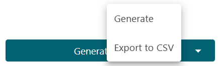
Alternatively, the results can be directly exported to a CSV instead of as a layer in the layer manager.
Instruction Video
Options
| Option | Description |
|---|---|
| Cable/pipeline | Selects the cable/pipeline. |
| Bathymetry layer A | Selects the layer with the seabed floor. |
| Bathymetry layer B | Selects the layer with the seabed floor. |
| Criteria | Selects the status for the difference levels. |
| KP | Optionally selects a section of the line instead of the full length of the line. This can be done with the slider or manually entering the start and end point. |
| Interval | Sets the interval for points in the line chart. The default is the KP points as defined on the cable/pipeline. It is also possible to set a fixed distance between the points. |
CSV output format
The CSV is in XYZ format, each point on a cable has its own row.
Example:
| CableName | X | Y | Z | KP | Difference | 2019 | 2020 | Status | Criteria |
| A1 | 444343.8 | 5965793 | 0 | 0 | -9.36 | Unknown | |||
| A1 | 444343.5 | 5965794 | 0 | 0.001 | -9.36 | Unknown | |||
| A1 | 444343.1 | 5965795 | 0 | 0.002 | -9.36 | Unknown | |||
| A1 | 444342.7 | 5965796 | -13.25 | 0.003 | 2.43 | -11.78 | -9.35 | Big positive | >= 1m |
| A1 | 444342.2 | 5965797 | -12.96 | 0.004 | 2.34 | -11.7 | -9.36 | Big positive | >= 1m |
| A1 | 444341.8 | 5965797 | -12.51 | 0.005 | 1.77 | -11.13 | -9.36 | Big positive | >= 1m |
Profile Tools
Overview of profile tools
With our range of Profile Tools you can visualize the raster and vector data (Z values) as a line or a point in a profile graph. Monopiles and/or cables are included in the profile at the correct location.
The tools depends on bathymetry (raster) layers, cable, pipeline or monopile (vector) layers. The application looks for layers that are marked as these object types. The Profile Tools automatically become available once these layers are found in the project.
When using profile tools be sure to set the correct Object type in Update Layer. To be able to see cable or pipeline profiles you must ensure the Object type is "with depth" for the depth to be visible in the tool
Tools
| Icon | |
 |
Cable/pipeline profile Create a profile over a cable or pipeline. Shows the cable or pipeline in relation to the seabed floor. |
 |
Map profile Create a profile over a line on the map. Can be used to create a cross section over a cable or pipeline. |
 |
Radial profile Create a profile of several lines across a point or monopile position. Can be used to monitor scour protection around a monopile. |
 |
Cable Protection System (CPS) profile Create a profile from a monopile to the nearest cable endpoints. |
Profile Chart
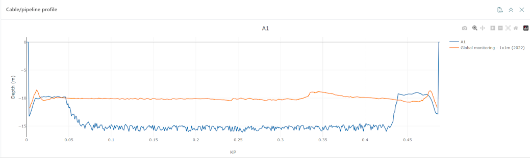
All of the above tools generate a profile chart at the bottom of the screen. The image above shows a cable (A1) and a bathymetry layer (Global monitoring - 1x1m (2022)). The y-axis of the chart shows the height of the cable/seabed. Hovering over a line in the chart gives the position and depth. A dot will also appear on the highlighted cable/pipeline on the corresponding position on the map.
With the blue icons on top it is possible to:
- Export the data of the profile to a CSV file for use in external applications.
- Expand or collapse the dialogue.
- Close the dialogue.
With the gray icons on top it is possible to:
- Create a snapshot and save it as an image.
- Zoom in and out. It is also possible to zoom in by drawing a box in the graph.
- Pan the profile to the left/right.
- Automatically scale.
- Reset the profile to its original view.
Clicking on a line in the legend will hide/show a line in the profile. Double-clicking on a line will single out the line and grey out the other information.
Cable/pipeline profile
This tool creates a profile showing the height of subsea cables and pipelines as recorded by surveys. The results are displayed in a single, convenient chart.
The tool, which creates a profile over a cable, automatically becomes available when the software detects the required layers with object type bathymetry and cable/pipeline in the project.
The dialogue can be triggered in two ways:
- From the right side menu on the map
- From the info panel when the selected feature has objecttype cable/pipeline or is a line feature. The profile icon appears in the action button bar.
Once selected a pop-up will appear on the right side of the map.
Options
| Option | Description |
|---|---|
| Cable/pipeline | A drop-down to select the target cable/pipeline. |
| KP | Once the cable/pipeline is selected, we can (optionally) select part of the cable/pipeline. This can be done by adjusting the slider or setting the start and/or end point manually. |
| Interval | Set the interval for points in the line chart. KP points as defined on the cable/pipeline are the default. It is also possible to set a fixed distance between the points. |
| Bathymetry | Selects the bathymetry layers to add to the line chart. Select ‘all' or ‘visible on map' bathymetry layers. |
Instruction Video
Map Profile
Create a profile from a line on the map. This can be a single straight line or contain several sub-sections. The line can be created in two ways:
- Drawing on the map: Under the cursor there is an orange point. Clicking once sets a point on the line. A double click ends the line and automatically generates a profile. Once the line has been created it is possible to drag the points to adjust the profile.
- Adding points in the dialogue: It is possible to manually set the XY coordinates of points in the options dialogue for precise control.
Options
| Options | Description |
| Line coordinates | Adds points to the line. Will be automatically set when a point is added by clicking on the map. |
| Interval | Sets the distance between the points in the graph. The default is one meter. |
| Bathymetry | Selects the bathymetry layers to add to the line chart. Select ‘all' or ‘only visible' bathymetry layers. |
Instruction Video
Radial Profile
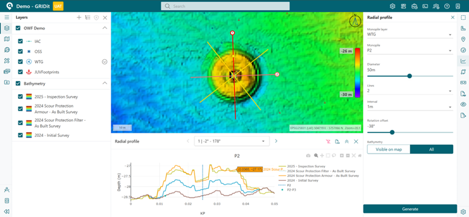
This tool allows GRIDit users to visualize the scour protection surrounding a monopile by creating a profile of several lines across a monopile position. The number of lines can be adjusted.
The dialogue can be triggered in two ways:
- From the right side menu on the map
- From the info panel when the selected feature includes a monopile. The profile icon appears in the action button bar.
Options
| Options | Description |
|---|---|
| Monopile layer | The layer with the monopile / feature. |
| Monopile | The monopile at the center of the radial profile. |
| Diameter | The diameter of each line across the center of the radial profile. |
| Lines | The number of lines in the profile. |
| Interval | Sets the distance between the points in the graph. The default is one meter. |
| Bathymetry | Selects the bathymetry layers to add to the line chart. Select ‘all' or ‘only visible' bathymetry layers. |
Profile chart
The generated profile chart has an extra drop-down menu to switch between the different lines. The selected line is highlighted on the map.
Instruction Video
Cable Protection System (CPS) Profile
The CPS Profile Tool allows users to monitor scouring around the Cable Protection System (CPS), the offshore wind asset that protects the cable between leaving the seabed and entering the monopile or J-tube.
With the CPS Profile Tool, users can configure profiles from the monopile up to (and including) the cable. Users select the profile length and interval.
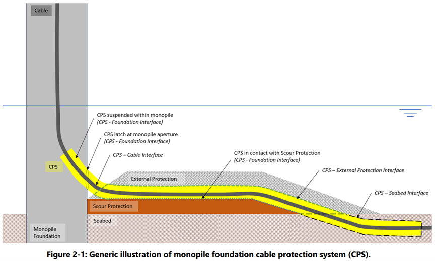
Source: Cable Protection Systems (CPS) best practice guideline / Carbon Trust Offshore Wind Accelerator (OWA), November 2024
Using the CPS Profile Tool
The dialogue can be triggered in two ways:
- From the menu on the right hand side of your GRIDit page. Select
 followed by
- From the info panel when the selected feature includes a monopile. The profile icon appears in the action button bar.

Options
| Options | Description |
|---|---|
| Monopile layer | The layer with the monopile feature. |
| Monopile | The monopile at the center of the radial profile. |
| Length | The length of the profile from the monopile. The default is up to the cable, but may be extended beyond. |
| Bathymetry | Selects the bathymetry layers to add to the line chart. Select either ‘all' or 'only visible' bathymetry layers. |
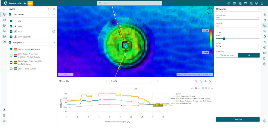
Profile Chart
The generated profile chart has a drop-down menu to switch between profiles. The selected profile is highlighted on the map in red (see below).
How does GRIDit generate the profile between the monopile and cable?
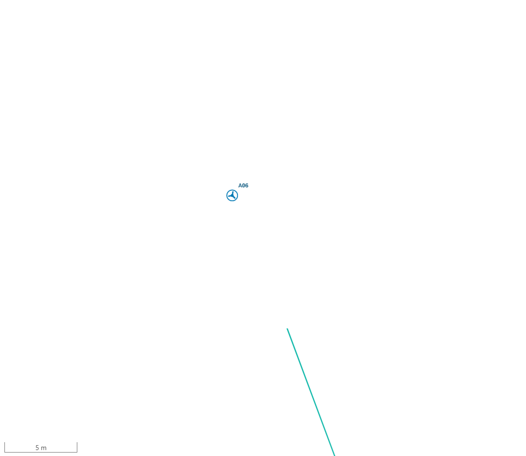
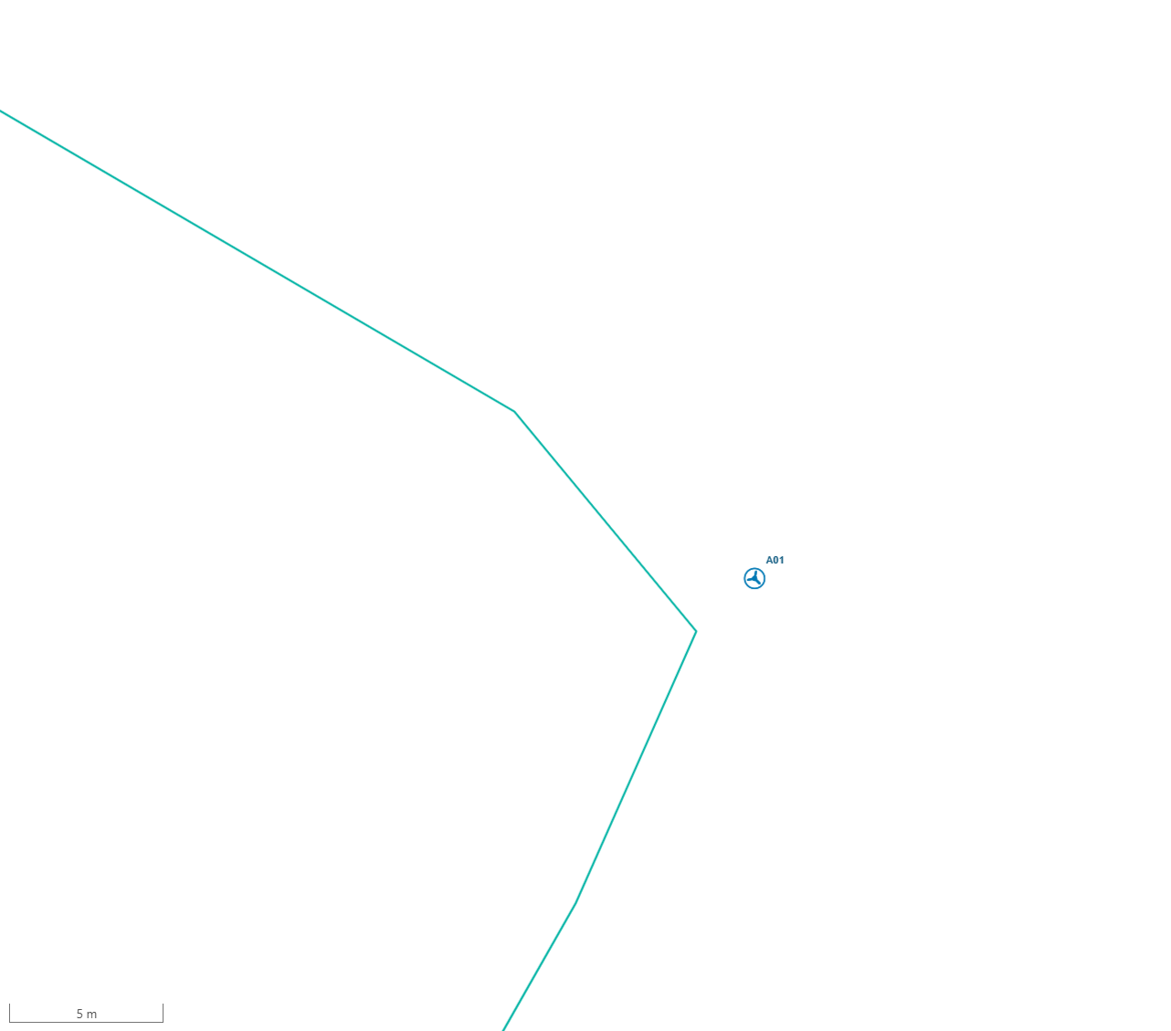
The CPS tool starts from the monopile location and extends a straight line to connect to the start/end point of a cable, this line forms the length of the generated depth profile. Once the line joins the cable, it will follow the cable as it curves. The start/end of the cable must be within 100 meters of the monopile for the CPS tool to find it. If a cable's data is continuous, the CPS tool will not be able to find a location generate a depth profile to. Here is an example to illustrate.
| Cable will be found, profile generated | Cable won't be found, no profile generated |
 |
 |
Calculate Tools
Overview of Tools
| Icon | Descriptions |
 |
Calculate the difference between a raster layer and a reference |
 |
Calculate the volume difference between bathymetry layers or against a reference level within defined polygon areas |
Calculate Raster
The Calculate Raster tool allows calculations to be made, either between two overlapping bathymetry layers, or between one bathymetry layer and a fixed value. This has many useful purposes, including allowing users to compare designs with the reality on the seabed.
When a calculation is made, a new layer is created.
All the basic arithmetic operations (add/subtract/divide/multiply/average) are supported.
Prerequisites:
- At least one bathymetry layer loaded in your project.
- One or more polygon features defining calculation area(s).
The Calculations menu is only available when you have at least one bathymetry layer in your project.
Options
| Option | Description |
|---|---|
| Mode | Layers Makes mathematical calculations between two bathymetry layers Fixed value Makes mathematical calculations between a bathymetry layer and a fixed value |
| Bathymetry layer A | The current situation |
| Bathymetry layer B | If mode = “layers" this is the reference layer/design |
| Fixed value | If mode = “fixed value" then this is the second parameter in the calculation operation |
| Operation | Add A + <layer B/value> Subtract A - <layer B/value> Divide A / <layer B/value> Multiply A * <layer B/value> Average (A + <layer B/value>) / 2 |
| Layer | The name of the layer to be created |
| Personal layer | Only possible for those with a contributor role. Select “Yes" visible to you |
| Layer group | Place the new layer in this layer group |
Instruction Video
Calculate Volume
The Calculate Volume tool calculates the volume difference within defined polygon areas between two bathymetry layers or against a reference level. This is commonly used for monitoring scour protection around monopiles and determining material volume/dredging requirements. The tool outputs into PDF or CSV format.
Quick Start
Prerequisites:
- At least one bathymetry layer loaded in your project.
- One or more polygon features defining calculation area(s).
The Calculations menu is only available when you have at least one bathymetry layer in your project.
Modes:
| Mode | Use When | Example |
| Reference Layer | Comparing two bathymetry surveys to detect changes over time or want to calculate volume to meet requirements after erosion | Comparing pre-installation seabed scan with current conditions around monopile foundation. |
| Reference Level | Calculating volume relative to a fixed elevation |
Calculating rock dump volume from a fixed level to the top of the rock dump. |
Example: reference layer
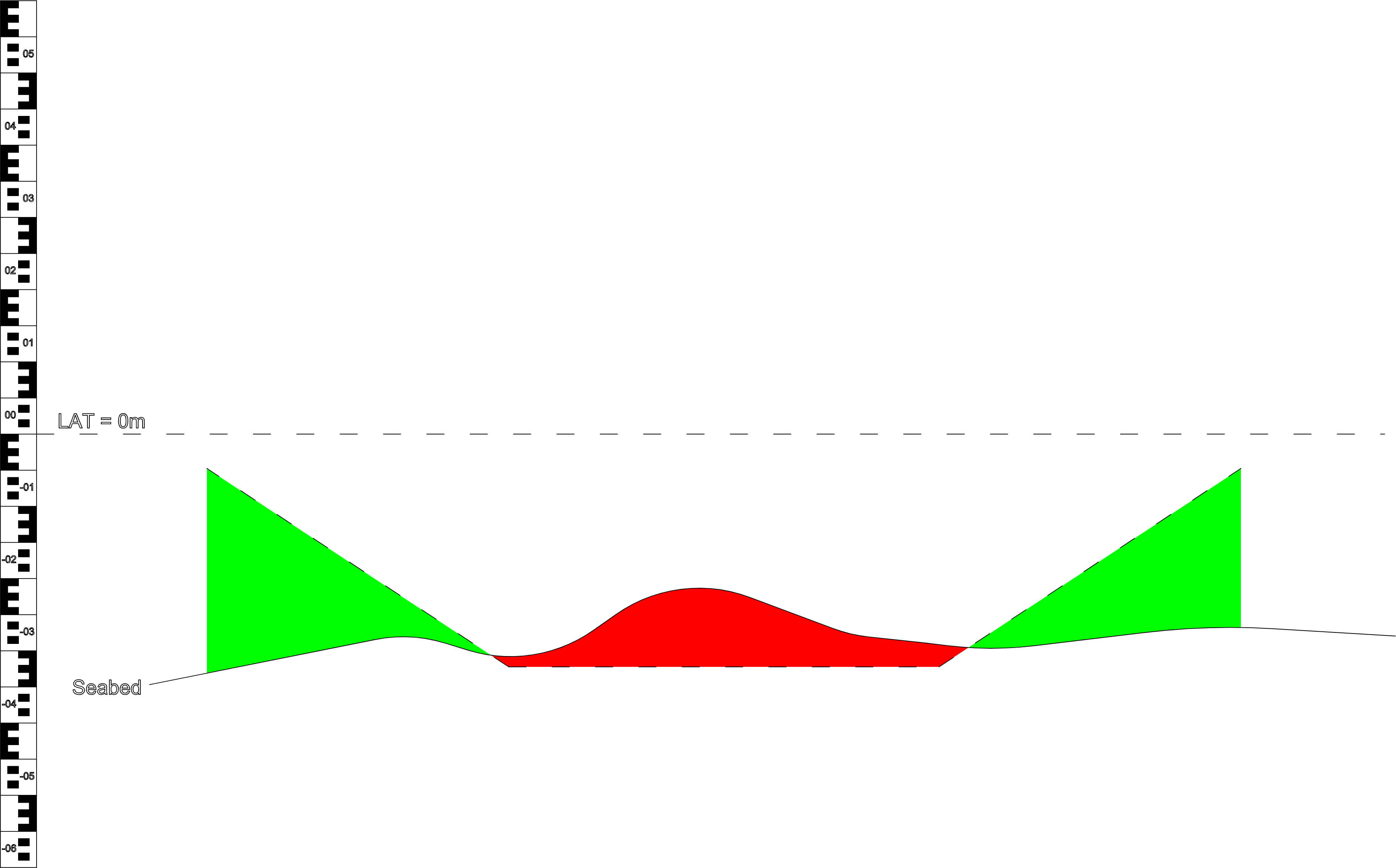
Example 1 - Design as the reference layer (vs Seabed)
Example 2 - Post Dredge Seabed as reference layer (compared with Pre Dredge Seabed)
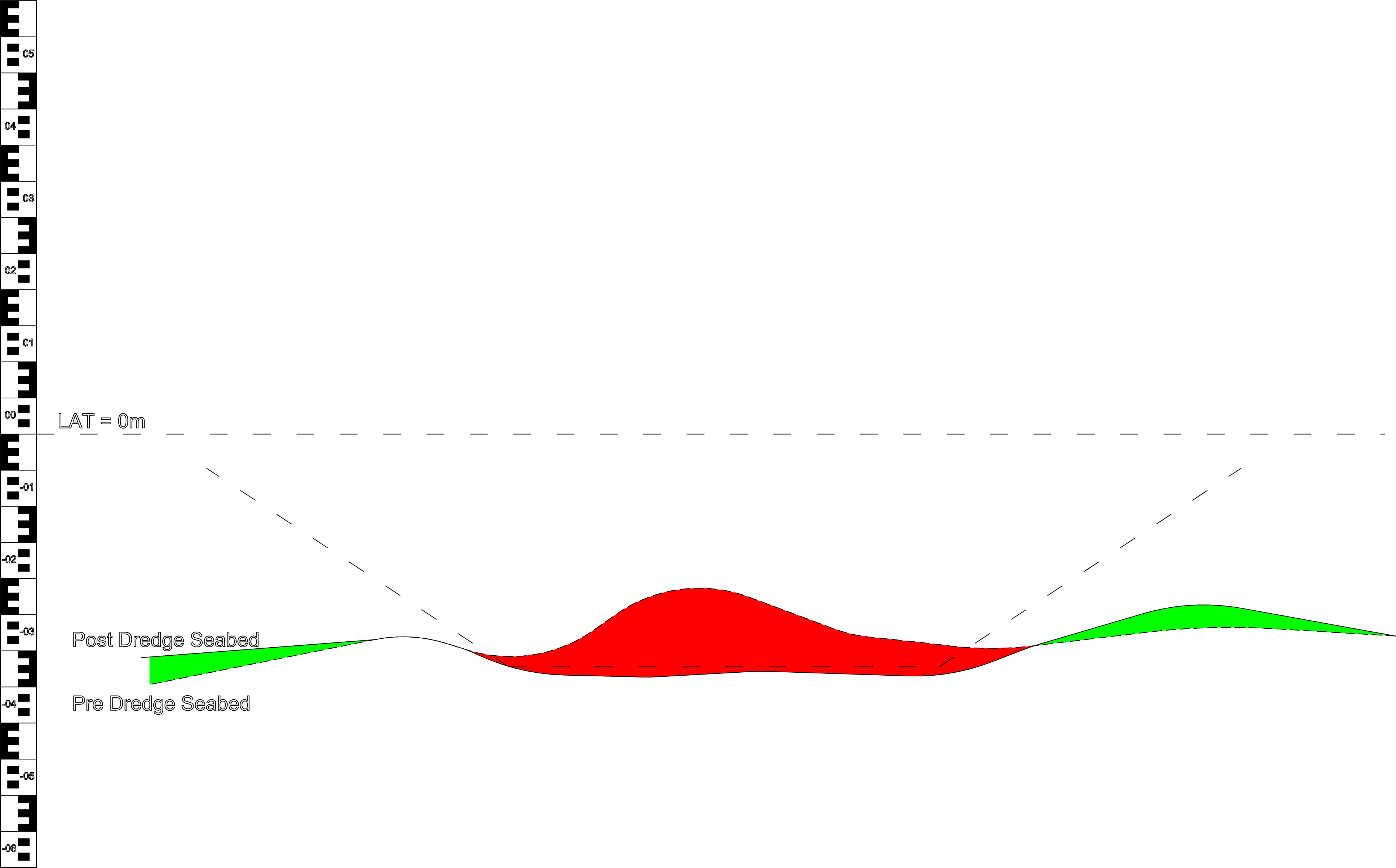
Red = Volume above the reference layer
Green = Volume below the reference layer
Example: reference level
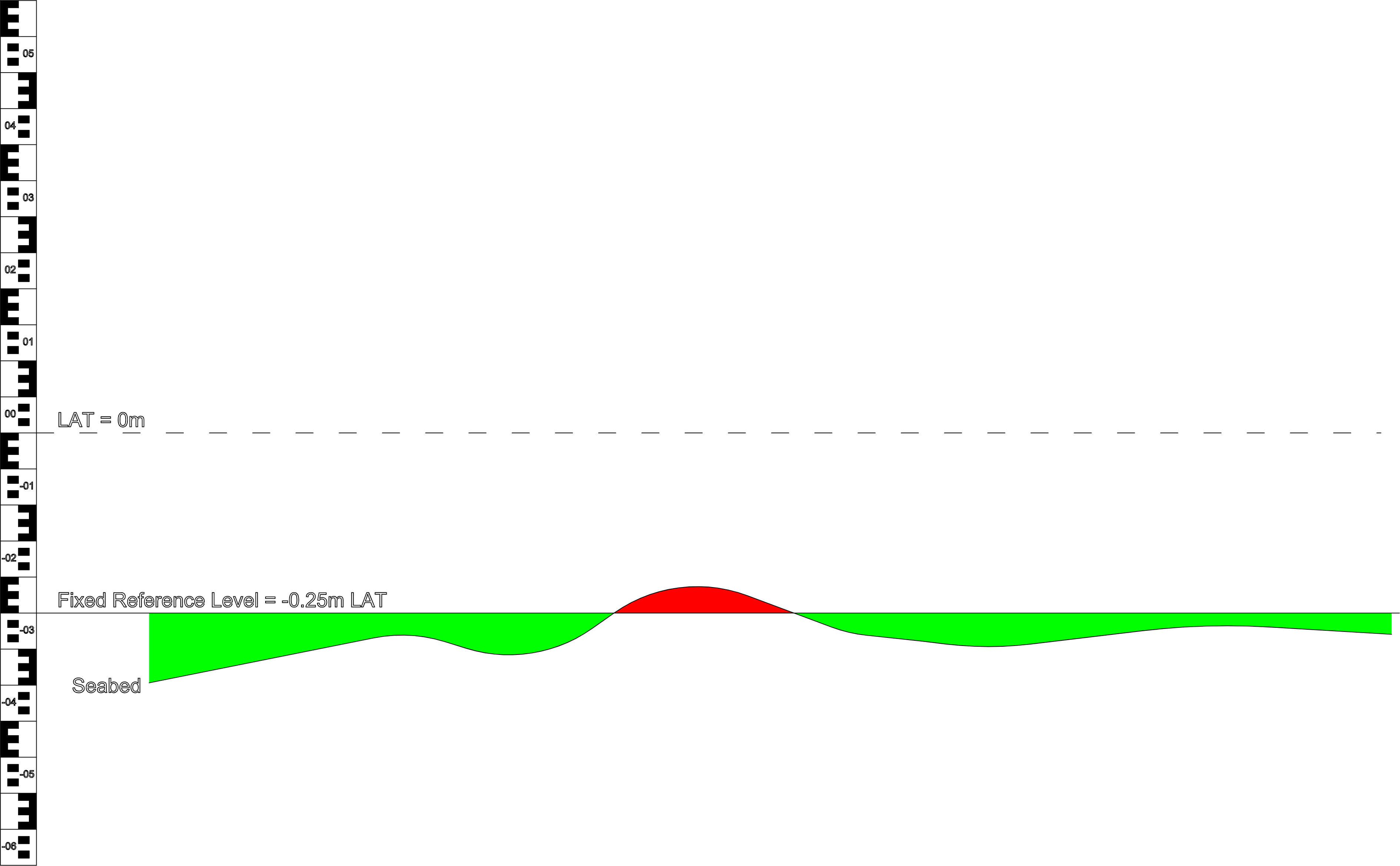
Red = Volume above the reference level
Green = Volume below the reference level
Basic workflow:
- Select a model layer (the bathymetry layer to analyze)
- Choose calculation mode (Layers or Reference Level)
- Select reference layer (Layers mode) or enter reference level in meters (Reference Level mode)
- Select polygon layer containing your areas of interest
- Choose one or more polygons to calculate volume for
- Click Export to CSV or Export to PDF
Layer terminology
| Layer | How to use |
| Model Layer | This is the baseline to which you will be comparing a design or DTM (digital terrain model) |
| Reference layer |
This is normally the design that you will be comparing to the model layer (baseline) |
| Reference level |
The depth level in relation to vertical reference that you will compare to the model layer (baseline) |
Understanding Results
How volume is calculated (nearest-neighbour resampling)
Nearest Neighbor is a method used to align two raster layers of different detail levels (resolutions) without changing the original data.
What happens in your project?
When comparing a 1x1m survey to a 0.25x0.25m model, or visa versa the volume calculator needs them to speak the same "language." Using Nearest Neighbor, it divides each large 1m cell into 16 smaller 0.25m cells.

Why use this calculation method for volumes?
- Zero Distortion: It doesn't "invent" new heights. It simply duplicates the measured 1x1m height into the smaller squares.
- Mathematical Purity: If your 1x1m square says the ground is at 10 meters, all 16 smaller squares will also be exactly 10 meters.
- Honest Comparison: Other methods (like "Bilinear") would try to smooth the edges, creating "fake" slopes between points. Nearest Neighbor ensures you are comparing your actual measurements directly against the reference model.
The Result
It’s like taking a large Lego brick and swapping it for 16 tiny ones of the same height. The total volume remains identical, but the grid now perfectly matches your high-resolution reference model.
Nearest Neighbor keeps data honest. It changes the 'grid size' without changing the 'measured value,' making it the safest choice for calculating volumes between different survey sources.
The volume calculation produces the following metrics for each selected polygon:
| Metric | Description |
|---|---|
| Model Name | The model layer that is being used to calculate volume for |
| Reference Name | The layer that is being used as the reference for the calculation |
| Polygon Name | The area for which volume will be calculated |
| Volume Above Reference (m³) | Volume where the model layer is higher than the reference (material addition or accumulation) |
| Volume Below Reference (m³) | Volume where the model layer is lower than the reference (material loss or erosion) |
| Volume Difference (m³) | Net volume change (Volume Above minus Volume Below). Positive values indicate net accumulation; negative values indicate net loss |
| Area Above Reference (m²) | Surface area where the model layer is above the reference |
| Area Below Reference (m²) | Surface area where the model layer is below the reference |
| Polygon Area (m²) | The area of the polygon (regardless of whether there is area with or without data) |
| Area without Data (m²) | Area inside the polygon which is not covered by the model layer (required to be able to calculate the average layer thickness) |
| Area without Reference (m²) | Area inside the polygon which is not covered by the reference layer (required to be able to calculate the average layer thickness) |
| Average Layer Thickness (m) |
Average heights of the layer that falls withing the polygon (and coverage with data and reference) |
All values are rounded to two decimal places in the output.
Tips and Best Practices
- Plan your polygon areas carefully: Create polygon layers that match your analysis needs before starting calculations. Well-defined areas of interest will make your workflow more efficient.
- Use meaningful layer names: Name your bathymetry layers with dates or survey identifiers to easily track which data you're comparing.
- Monitor calculation time: Calculations on large areas or high-resolution data may take some time. The tool displays a loading indicator during processing.
- Export both formats: Consider exporting both CSV and PDF formats—CSV for detailed analysis and PDF for documentation and reporting.
- Interpret Volume Difference carefully: Positive values indicate net accumulation; negative values indicate net loss. This metric is particularly useful for quick assessment of material changes.
- Use map highlighting: Selected polygons are highlighted on the map and automatically centered in the view, making it easy to verify you're analyzing the correct areas.
- Keep data organized: Maintain a clear naming convention for your surveys and regularly export calculation results to track changes over time.
Detailed guide
The Calculate Volume tool enables you to calculate volumetric differences in bathymetric data (bathymetric layers) within specified areas (polygons). This functionality is essential for monitoring seafloor changes, particularly for offshore wind farm applications where scour protection monitoring around monopile foundations is critical.
The tool calculates volumes in cubic meters and areas in square meters, providing detailed metrics including volume above, volume below, and net volume difference for each selected polygon.
Prerequisites
Before using the Calculate Volume tool, ensure you have:
- Bathymetry layers: At least one bathymetry layer loaded in your project. To Layers mode, you need at least two compatible bathymetry layers.
- Polygon layer: A feature layer containing polygons that define the areas where you want to calculate volumes.
- Overlapping data: The model layer and reference (layer or polygons) must have overlapping geographic extents.
The Calculations menu is only available when you have at least one bathymetry layer in your project.
Configuration
1. Mode selection
| Mode | When to use? |
| Reference layer |
Use this mode when you want to compare two bathymetric surveys to calculate changes over time or want to calculate volume to meet requirements after erosion. This is ideal for:
|
| Reference level (m) |
Use this mode when you want to calculate volume relative to a fixed elevation value. This is useful for:
|
2. Model Layer Selection
The model layer is the primary bathymetry layer you want to analyze. This is typically your most recent survey or the layer representing current conditions.
Select your model layer from the Model layer dropdown menu. Only bathymetry layers that are ready for calculations will be available in this list.
Important: Once you select a model layer, the tool automatically filters the available reference layers and polygon layers to show only those that are compatible (matching projection and overlapping geographic extent).
3. Reference Selection
The reference defines what your model layer will be compared against. The reference selection depends on your chosen mode:
For Layers Mode:
Select a reference layer from the dropdown. This should be your baseline bathymetry survey, typically an earlier survey that you want to compare against.
Only bathymetry layers that have overlapping coverage will appear in this list.
For Reference Level Mode:
Enter a reference level value in meters. This value represents the elevation you want to use as your comparison baseline.
- Positive values: Measure upward from the seabed (e.g., +2.0 meters above the seabed surface)
- Negative values: Measure downward from the seabed (e.g., -10.0 meters below the seabed surface)
Example: For a scour protection mound where you want to calculate the volume from the top down to 10 meters below the peak, you would enter -10.0 as your reference level.
4. Polygon Layer Selection
Select the feature layer that contains the polygons defining your areas of interest. These polygons specify the area for which the volume calculations will be performed.
Only layers containing polygon or closed line string features that overlap with your model layer will be available in the Polygon layer dropdown.
5. Polygon Selection
After selecting a polygon layer, choose which specific polygons you want to include in the calculation:
- Click the Polygons dropdown to see all available polygons from the selected layer
- Select one or more polygons (multi-select is supported)
- Use the Select All option to quickly select all available polygons
Selected polygons will be highlighted on the map, and the map view will automatically zoom to show all selected areas.
do we need to explain what could be the problem if they do not see any polygons (again)? I'm assuming they did not read above.
Exporting the results
The Calculate Volume tool offers two export formats:
CSV Export
Exports calculation results as a comma-separated values file suitable for:
- Import into spreadsheet applications (Excel, Google Sheets)
- Further data analysis and processing
- Integration with other software tools
- Creating custom reports or visualizations
PDF Export
Generates a PDF report with one page per selected polygon, each containing:
- A table with all calculation metrics for that polygon
- A map view centered on the polygon area with bathymetry data
The PDF format is ideal for documentation, presentations, and sharing results with stakeholders who don't need to manipulate the data.
To export:
- Click the main export button to use the currently selected format (default is CSV)
- Or click the dropdown arrow to choose between CSV and PDF formats
- The file will be automatically downloaded with a filename based on your model layer name
Common Use Cases
Scour Protection Monitoring
Scenario: You need to monitor the scour protection around monopile foundations and determine if additional material needs to be placed.
Approach:
- Use Layers mode to compare your recent survey (model layer) against the as-built survey, previous monitoring survey or design (reference layer).
- Select polygons around each monopile location.
- Export results to identify locations with negative volume difference (material loss) that may require remediation.
Rock Dump Volume Estimation
Scenario: You need to estimate the volume of rock material in a scour protection mound using a fixed reference level (-10m).
Approach:
- Use Post survey model layer and a fixed level as reference
- Enter -10.0 as the reference level (10 meters below the surface)
- Select the polygon encompassing the rock dump area
- The Volume Above value will represent the amount of material to dump
Change Detection Analysis
Scenario: You need to assess changes across multiple locations between two survey periods.
Approach:
- Use Layers mode with your newer survey as the model layer and older survey as the reference layer
- Select all polygons of interest using the Select All option
- Export to CSV for analysis in spreadsheet software
- Sort by Volume Difference to quickly identify areas with the greatest changes
Troubleshooting
Layer options are limited after selecting model layer
This is expected behavior. The tool automatically filters available layers to show only those that are compatible with your selected model layer (same projection for reference layers, overlapping extent for polygon layers).
Error: Bathymetry layer(s) are missing the required data file
This error occurs when one or more selected bathymetry layers don't have the necessary processed data for calculations. Ensure that your bathymetry layers have been fully processed before attempting volume calculations.
Unexpected or incorrect results
If results seem incorrect:
- Verify that both layers (in Layers mode) use the same coordinate reference system
- Confirm that your polygons actually overlap the bathymetry data coverage area
- Check the vertical reference system of your bathymetry layers
- In Reference Level mode, verify you've entered the reference level with the correct sign (positive or negative)
Markers
The Marker tool allows users to mark a location/POI to the map with notes. The notes have two properties: title and description.
The points are added to an existing marker layer. A new one will be created if none exists. Once created, it behaves like a standard vector layer. Styling can be adjusted, the data can be modified or exported, and media files can be attached.
The position of the marker on the map can be set in the dialogue or by clicking on the map. A click on the map sets the X and Y position in the dialogue.
Once a marker layer has been created the marker icon is visible to the right of the layer name. The layer can be edited, shared and exported just like other layers.

Options
| Option | Description |
| Title | The title of the marker (prefilled with marker). |
| Description | An optional and additional note. |
| X | The x position on the map. |
| Y | The y position on the map. |
| Layer | The name of the layer for the marker. This can be a new or existing layer. The plus sign allows the user to set a layer group for the layer. |
| Layer group | Additional option to set the layer group for the layer. |
3D View
The 3D Visualization tool allows the XYZ data to be examined as a pointcloud in a new browser tab. Users can by view, rotate, zoom in and zoom out.
The option can be loaded from the layer context menu. A layer can also be selected and loaded in the dialogue if the 3D view is selected in the right-side tool bar.
Instruction Video
Export Map to PDF
Users can download a section of the map as a PDF. This tool can be used to print out any details from the project. Once the ‘Export Map' button is clicked, a menu will be displayed along with a rectangle on the map. The rectangle, which indicates the area on the map to be exported, can be moved.
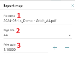
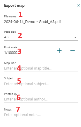
Depending on whether an A3 or A4 format is selected, the menu will appear as follows:
| Menu A4 | Menu A3 (Default) |
 |
 |
Options
| Option | Description |
| 1. File name | The name of the file that will be downloaded when generate is clicked. |
| 2. Page Size | A dropdown menu to select the desired page size. |
| 3. Print Scale | The print scale is used to set the scale for the PDF. Changing the value of the scale will change the size of the rectangle on the map. |
| 4. Map Title (A3) | Add an optional chart title. |
| 5. Subject (A3) | Add a subject (optional). |
| 6. Printed By (A3) | Displays the name of who creates the map in the PDF. |
| 7. Notes (A3) | A place to add any additional notes. |